Vector Retrieval

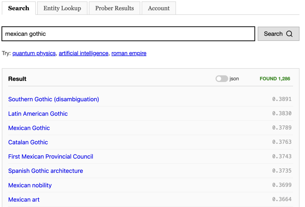
Now that every document has been assigned a vector encoding its semantics, this opens the door to a new kind of retrieval. Rather than find documents that might be relevant to the query by searching through the search index for keywords, we can instead take the query’s vector and find nearby documents in the embedding.

One advantage this has over keyword retrieval is that we know that all the documents we retrieve this way are on the right topic. So rather than going through tens of thousands of documents and scoring them, they come pre-scored by the embedding and so we need a lot fewer of them. Right now, the byte64 search engine is setup to pull only the 50 nearest neighbour documents to the query’s vector. And the results are great.

Let’s talk about the infrastructure that supports this kind of retrieval. The fundamental problem of exact vector-based nearest neighbour retrieval is roughly linear in the worst case. Approximate methods can speed this up considerably. Off the shelf, you can get Google’s Scaleable Nearest Neighbor library which provides everything you need — building an index and serving that’s optimized for x86 architecture. It can pull the nearest 50 documents in under 30ms. But for the wikipedia dataset, it costs another 4 GiB of ram.

I tried rolling my own approximate nearest neighbour algorithm. My idea was do divide the vectors in $\mathbb{S}^{127} = \{ v \in \mathbb{R}^{128} \mid \|v\| = 1\}$ into different cells $C_{ij}$. Then given a query vector $q \in \mathbb{S}^{127}$ we’ll select some cells that we think the candidates lie in. If the vectors within the cells are nicely ordered, we can even merge them using using a heap until we get the number of documents we want.

Given a vector $v = (v_1, \ldots, v_{128})$ let $v_i$ and $v_j$ be the largest and second largest component of v (taken in absolute values). We define $C_{ij}$ to be the collection of all such vectors — actually we need to account for the signs of $v_i$ and $v_j$ so we really need $C_{ij}^{++}, C_{ij}^{-+}, C_{ij}^{+-}, C_{ij}^{–}$. So, this defines $4 \cdot 128 \cdot 127$ different cells.

When we’re trying to find vectors near $q = (q_1, \ldots, q_{128})$, we sort the components in absolute values as $|q_{\sigma(1)}| \geq |q_{\sigma(2)}| \geq \cdots \geq |q_{\sigma(128)}|$ and then search in $C_{\sigma(1)\sigma(2)}^{s_1 s_2}, C_{\sigma(1)\sigma(3)}^{s_1 s_3}, C_{\sigma(1)\sigma(4)}^{s_1 s_4}, \ldots$in that order. Here $s_i$ is the sign of $q_{\sigma(i)}$.

I sorted the elements in $C_{ij}$ by their i-th component followed by j-th component, I was hoping next nearest neighbour would appear in $C_{\sigma(1)\sigma(k)}^{s_1 s_k}$ before $C_{\sigma(1)\sigma(k+1)}^{s_1 s_{k+1}}$. But unfortunately, the largest component isn’t the best indication of where the largest dot-product will be.

Take a look at the distribution of cosine similarities with an arbitrary nut-based wikipedia page.

Cosine Similarity Distribution (against page: https://en.wikipedia.org/wiki/Pistachio):
Bucket Range         | Count     
---------------------|-----------
[-1.00, -0.90) | 0
[-0.90, -0.80) | 0
[-0.80, -0.70) | 0
[-0.70, -0.60) | 0
[-0.60, -0.50) | 0
[-0.50, -0.40) | 0
[-0.40, -0.30) | 22
[-0.30, -0.20) | 2263
[-0.20, -0.10) | 49199
[-0.10,  0.00) | 343893
[ 0.00,  0.10) | 1018456
[ 0.10,  0.20) | 1997144
[ 0.20,  0.30) | 2221347
[ 0.30,  0.40) | 955750
[ 0.40,  0.50) | 318725
[ 0.50,  0.60) | 204906
[ 0.60,  0.70) | 18468
[ 0.70,  0.80) | 96
[ 0.80,  0.90) | 0
[ 0.90,  1.00) | 1

But if we use the approach above to retrieve the 10000 nearest neighbors of the document, we get this distribution:

Similarity Distribution of top 10000 results:
Bucket Range         | Count     
---------------------|-----------
[-1.00, -0.90) | 0
[-0.90, -0.80) | 0
[-0.80, -0.70) | 0
[-0.70, -0.60) | 0
[-0.60, -0.50) | 0
[-0.50, -0.40) | 0
[-0.40, -0.30) | 0
[-0.30, -0.20) | 0
[-0.20, -0.10) | 0
[-0.10,  0.00) | 0
[ 0.00,  0.10) | 0
[ 0.10,  0.20) | 0
[ 0.20,  0.30) | 0
[ 0.30,  0.40) | 0
[ 0.40,  0.50) | 0
[ 0.50,  0.60) | 5757
[ 0.60,  0.70) | 4203
[ 0.70,  0.80) | 39
[ 0.80,  0.90) | 0
[ 0.90,  1.00) | 1

So, we didn’t even retrieve half of the documents in the 0.7 to 0.8 range and those are all within the 100 nearest neighbours. This is pretty crumby recall, so I’m sticking with ScaNN for now.

Two downsides to ScaNN is that it uses a python frontend to a C++ backend and it also requires x86. This complicates testing, since it requires docker on Mac M and it means python is needed on the search server. These kind of algorithms are incredibly fun to learn and write. Since it’s open source, I’d love to port it to rust if I can.

~Andrew